What do we mean by modelling? There are different kinds of models. There are mathematical models and statistical models. And then we have some other models.
When we speak about models, we mean a representation of the thing we are interested in. Models share some features with the ‘real thing’, e.g. model aeroplanes can fly and look like real aeroplanes. However, they are a simplification and do not have all the features of the ‘real thing’. For example, these model aeroplanes cannot carry people. Models have some advantages: even though they can crash like a real aeroplane, model aeroplanes are less likely to hurt people in the process; and, because they are simpler, they are easier to understand and fix.
Mathematical and statistical models, in analogy to the model aeroplanes, are a simplified representation of a complex system we would like to understand. These models are not meant to represent the original system exactly but should provide useful abstractions. Their value is that they are easier to study and understand than the real system. Since models necessarily simplify reality, they are usually good for studying certain aspects of the real system but they fail at explaining other features. The art of modelling is therefore to come up with a simple representation that helps you understand the particular aspect you are interested in. To go back to the analogy of model planes: if you are interested in understanding aerodynamics, a disconnected wing may give you answers to some questions and a toy aeroplane with the right shape and proportions may give you answers to other questions. If you want to learn to fly a real aeroplane, a simulator may be a better model for you.
Likewise, you need to choose the appropriate mathematical and statistical model to answer your question. The eminent statistician George Box famously said “All models are wrong but some are useful”. Remember this quote. The conclusions you will draw from data always also depend on the models you used to obtain your results. It is incorrect to say “my data show…”. You can say “in the light of my model, the data show…”. As a data analyst, you will hear people complain that your model is wrong. Of course it is wrong; it is meant to be. If reality was simple you would not need a model to understand it and if your model is as complex as reality, it won’t help you understand anything. However, you are responsible for ensuring that your model is useful. This is in no way guaranteed.
What is a Model?
A statistical model is a mathematical representation of how data is generated. It describes the relationship between observed data and underlying factors (parameters) while accounting for random variation. Suppose that we are interested in estimating the age of a tree from its stem diameter. To do this we need to know by how much the stem diameter increases per year. We could describe this relationship or process as follows:
\[D = \alpha + \beta \times Age\] describing a linear increase of diameter with age. Once we have a good idea of how fast diameter increases with age (β) we can predict diameter from age. The (mathematical) model above is a very simple representation of this process with only two parameters, the intercept and the growth rate.
With the chosen parameter values, diameter increases linearly with age. Of course, this model is not realistic except for special situations but it gives us powerful insights. In reality we don’t know \(\beta\), but usually need to estimate it from data. Also, not every tree grows equally fast, because of environmental and individual differences between trees. We can accept that the above is a simple model for the average behaviour of a tree, but to capture variability between trees (because of variability between environmental conditions from tree to tree, variability between individual trees, measurement error), we add an error term.
\[D = \alpha + \beta \times Age_i + e_i\]
The response that we observe is then described by an average behaviour, but the actual observed value will vary around this average. To summarise, the statistical model has a stochastic component which captures variability in the response that cannot be explained by the deterministic part of the model. Another distinguishing feature of statistical modelling is that we obtain estimates of the parameter values from the data, e.g. by fitting a line to the observations, i.e. we learn from data.
Steps in statistical modelling
Statistics is an integral part of the scientific method and should be involved in all parts of the scientific process. A summary of the steps involved in scientific research:
Interesting scientific question.
Come up with a number of working hypotheses.
Plan / design study / experiment.
Data collection: field, experiment, observations.
Analysis: confront hypotheses with data.
New scientific questions, update working hypotheses.
More generally
Statistical models are not perfect predictors of the data, rather they attempt to describe the “central tendency” of the observations. To get to the actual observed value some deviation from the central tendency needs to added (i.e. error). Such models typically have the following the form:
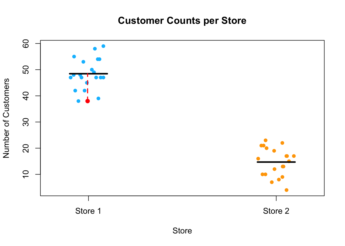
A simple example of a statistical model you may have encountered is the mean as a predictor. Suppose you measure the number of customers entering two stores over 20 days. The observed counts for each store fluctuate daily, but you may want to summarize the data using the average number of customers.
For each store \(i\), a basic statistical model for these observations would be:
\[
Y_{ij} = \mu_i + e_{ij}
\]
where:
\(Y_{ij}\) is the number of customers observed on day \(j\) at store 1,
\(\mu_i\) is the true mean number of customers at store \(i\),
\(e_{ij}\) is the error term, representing deviations from the mean.
The error term \(e_{ij}\) accounts for day-to-day fluctuations that cause the actual number of customers to vary around the mean. Below this data is simulated and plotted, with the model overlain. The black line is the mean and the red dashed line represents the error for one observation, i.e. deviation from the fitted model response, in this case the mean.
Code
store1 <-rpois(20, 50)store2 <-rpois(20, 15)storedata <-data.frame(numcust =c(store1, store2),store =factor(rep(c("Store 1", "Store 2"), each =20)))stripchart(numcust ~ store, data = storedata,method ="jitter", pch =16, col =c("deepskyblue", "orange"),vertical =TRUE, main ="Customer Counts per Store",xlab ="Store", ylab ="Number of Customers")means <-tapply(storedata$numcust, storedata$store, mean)segments(x0 =1:2-0.1, x1 =1:2+0.1, y0 = means, y1 = means, lwd =3, col ="black") min_count <-min(storedata$numcust[storedata$store =="Store 1"])min_x <-jitter(rep(1, sum(storedata$numcust == min_count))) points(min_x, min_count, col ="red", pch =16, cex =1.2) segments(x0 = min_x, x1 = min_x, y0 = min_count, y1 = means["Store 1"], col ="red", lwd =2, lty =2)
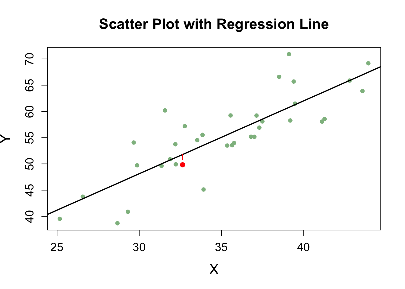
Another basic example of this structure is a linear regression model:
\[
Y_i = \beta_0 + \beta_1 X_i + e_i
\]
where:
\(Y_i\) is the observed response,
\(\beta_0\) and \(\beta_1\) are unknown parameters representing the intercept and slope,
\(X_i\) is the predictor variable,
\(e_i\) is the random error term.
Code
# Generate random x values and error termset.seed(123) # Ensures reproducibilityx <-rnorm(35, mean =35, sd =5)error <-rnorm(35, mean =0, sd =5)# Define true model parametersbeta0 <-2beta1 <-1.5# Generate y values based on the regression modely <- beta0 + beta1 * x + error# Fit a linear regression modelmodel <-lm(y ~ x) # This was missing!# Select an observation to highlightobs_index <-20x_obs <- x[obs_index]y_obs <- y[obs_index]y_pred <-predict(model, newdata =data.frame(x = x_obs)) # Scatter plot of data pointsplot(x, y, pch =16, col ="darkseagreen",xlab ="X", ylab ="Y",main ="Scatter Plot with Regression Line",cex.lab =1.5, cex.axis =1.2, cex.main =1.5)# Add regression lineabline(model, col ="black", lwd =2)# Highlight the observed pointpoints(x_obs, y_obs, col ="red", pch =16, cex =1.2) # Draw a dashed vertical line from the predicted value to the observed valuesegments(x0 = x_obs, x1 = x_obs, y0 = y_pred, y1 = y_obs, col ="red", lwd =2, lty =2)
Notation
When we fit the model to our data, we estimate the unknown parameters using observed data. We denote these estimates using hat notation to distinguish them from the true (but unknown) population parameters:
\[
\hat{\beta}_0, \quad \hat{\beta}_1
\]
Similarly, the fitted values (model-predicted responses) are denoted as: