par(mfrow = c(1,2))
plot(model, which = 1)
plot(model, which = 2)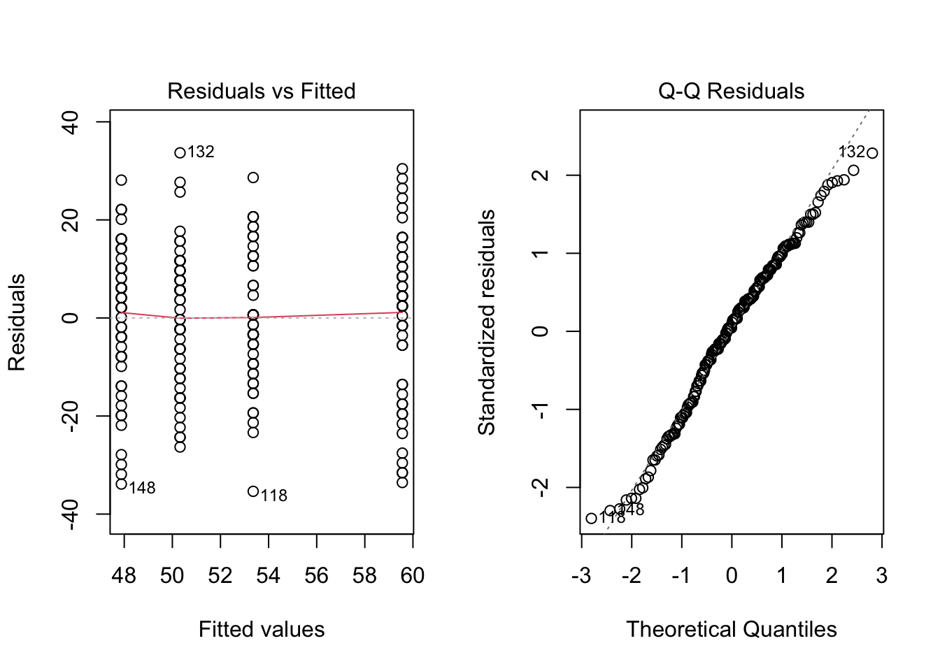
The model for a factorial experiment with two treatment factors was:
\[ Y_{ijk} = \mu + A_i + C_j + (AC)_{ij} + e_{ijk} \]
If we move \(\mu\) to the left-hand side of the equation, we get:
\[ Y_{ijk} - \mu = A_i + C_j + (AC)_{ij} + e_{ijk} \]
Now, each of the terms on the RHS is a deviation from a mean.
We can square and sum the corresponding observed deviations and obtain sums of squares. For a balanced factorial experiment, the total sum of squares on the LHS can be split into four parts, corresponding to:
\[ SS_{total} = SS_A + SS_C + SS_{AC} + SS_E \]
The degrees of freedom for these sums of squares are:
\[ abn - 1 = (a - 1) + (b - 1) + (a - 1)(b - 1) + ab(n - 1) \]
where \(n\) is the number of replicates per treatment. The degrees of freedom on the right-hand side add up to the total degrees of freedom. Once again, we summarise all this in a table.
The following table summarizes the partitioning of variation:
| Source | SS | df | MS | F |
|---|---|---|---|---|
| A Main Effects | \(SS_A = nb \sum_i (\bar{Y}_{i..} - \bar{Y}_{...})^2\) | \((a - 1)\) | \(MS_A\) | \(\frac{MS_A}{MS_E}\) |
| C Main Effects | \(SS_C = na \sum_j (\bar{Y}_{.j.} - \bar{Y}_{...})^2\) | \((b - 1)\) | \(MS_C\) | \(\frac{MS_C}{MS_E}\) |
| AC Interactions | \(SS_{AC} = n \sum_{ij} (\bar{Y}_{ij.} - \bar{Y}_{i..} - \bar{Y}_{.j.} + \bar{Y}_{...})^2\) | \((a - 1)(b - 1)\) | \(MS_{AC}\) | \(\frac{MS_{AC}}{MS_E}\) |
| Error | \(SS_E = \sum_{ijk} (Y_{ijk} - \bar{Y}_{ij.})^2\) | \(ab(n - 1)\) | \(MSE\) | - |
| Total | \(SS_{total} = \sum_{ijk} (Y_{ijk} - \bar{Y}_{...})^2\) | \(abn - 1\) | - | - |
There are three F-tests in this ANOVA table.
The alternative hypothesis is, in each case, that at least one of the parameters considered is non-zero.
While discussing interactions, we saw that sometimes, with strong interaction effects, the main effects of a factor may disappear (be close to zero). But this does not mean that the factor has no effect. On the contrary, it has an effect on the response; the effects just differ over the levels of the other factor and may average out.
Therefore, we usually start by testing the interaction effects. If there is evidence for the presence of interactions, we have to examine the main effects with this in mind, i.e., be careful with the interpretation of the main effects. Some people say that it becomes meaningless to test for main effects if there is evidence of interactions. However, this depends on what we want to know. The main effects still tell us whether or not the average response changes with changing levels of the factor.
The F-ratio always has the mean square for error in the denominator. As before, it is a ratio of two variance estimates, and in each case, it can be seen as a signal-to-noise ratio: how large are the effects relative to the experimental error variance?
Before we inspect the ANOVA table for the working example, we need to check the assumptions about the errors after model fitting. We do this by inspecting the residuals.
par(mfrow = c(1,2))
plot(model, which = 1)
plot(model, which = 2)
There are no clear violations, in the first plot, the residuals appear to be centered around zero and the spread is reasonably equal across groups. The second plot is a Q-Q plot of the residuals which shows nothing worrisome. Remember we can also plot a histogram of the residuals to check normality.
For the independence assumption, we construct the dot chart once again but with the residuals.
dotchart(model$residuals) # note the different way of extracting residuals!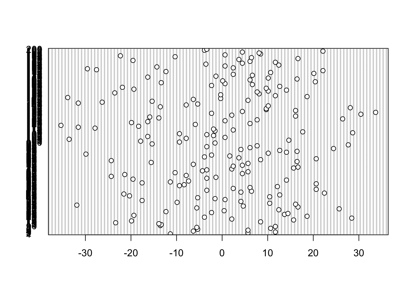
The y-axis is messy but we can ignore that, it shows the index of each observation and there are 200 hence why it overlaps so much. The residuals look uniform, there are no systematic patterns or trends in the plot.
Let’s see what the ANOVA table looks like for our working example.
summary(model) Df Sum Sq Mean Sq F value Pr(>F)
Speed 1 933 933.1 4.201 0.041724 *
Content.Type 1 2708 2708.5 12.195 0.000592 ***
Speed:Content.Type 1 177 176.7 0.796 0.373485
Residuals 196 43532 222.1
---
Signif. codes: 0 '***' 0.001 '**' 0.01 '*' 0.05 '.' 0.1 ' ' 1Verify that the degrees of freedom are what you expected! First, we look at the interaction. The F-value is quite small which leads to a large p-value of 0.37. This means that we really have no evidence against the null hypothesis that the factors interact. There is some evidence for a main effect of Speed but there is much stronger evidence as indicated by the small p-value for a main effect of lecture modality.